Introduction
The Generalized Method of Moments (GMM) is a powerful and flexible estimation method widely used in econometrics, especially for panel data and structural models. Developed by Lars Peter Hansen in 1982, GMM allows researchers to estimate parameters without fully specifying the distribution of the data, relying instead on moment conditions derived from economic theory or statistical properties.
In this blog post, we’ll demystify the intuition behind GMM. We’ll start with what moment conditions are, move on to identification, and then unpack the mechanics of GMM estimation. Finally, we’ll look at code examples in both R and Python to help you get hands-on experience.
Let’s get started.
What Are Moment Conditions?
Intuition First
Before diving into math, think of moment conditions as equations that should hold true if your model is correct.
For example, if you’re modeling a simple linear regression:

Assuming εi has zero mean and is uncorrelated with xi, the following condition must hold:

This is a moment condition — a statement about an expectation being zero.
Formal Definition
A moment condition is a function g(Zi,θ) such that:

- Zi is your data (could be xi,yi, instruments, etc.)
- θ0 is the true parameter value
- g(⋅) is usually a vector-valued function
GMM estimation finds the value of θ that makes the sample analog of this expectation as close to zero as possible.
Identification in GMM
What Does It Mean to Be Identified?
A parameter θ is identified if there is one and only one value of θ\thetaθ that makes the moment conditions true in the population.
If you have as many moment conditions as parameters, and they are linearly independent, the model is just identified.
If you have more moment conditions than parameters, the model is over-identified.
Over-identification allows you to test whether your instruments or model assumptions are valid using a J-test.
Mechanics of GMM Estimation
Step 1: Define Sample Moments
You replace expectations with sample averages:

Step 2: Choose a Weighting Matrix
The GMM estimator minimizes:
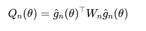
where Wn is a positive semi-definite weighting matrix.
- In just-identified models, the choice of Wn doesn’t matter.
- In over-identified models, the optimal choice is Wn=S^{-1}, the inverse of the covariance matrix of the moment conditions.
Step 3: Solve the Optimization Problem
This requires numerical optimization.

GMM in Action: Code Examples
Let’s estimate a simple linear model using GMM in R and Python.
Suppose our true model is:
We assume:
- E[xi⋅εi]=0
- So, moment condition: E[xi(yi−βxi)]=0
We’ll simulate some data and estimate β using GMM.
R Code:
library(gmm)

# Simulate data
set.seed(123)
n <- 1000
x <- rnorm(n)
beta_true <- 2
eps <- rnorm(n)
y <- beta_true * x + eps

# Define moment function
moment_fun <- function(theta, data) {
  x <- data[, 1]
  y <- data[, 2]
  g <- x * (y - theta[1] * x)
  return(matrix(g, ncol = 1))
}

data_mat <- cbind(x, y)

# Estimate using GMM
gmm_model <- gmm(g = moment_fun, x = data_mat, t0 = c(1))
summary(gmm_model)
Python Code:
import numpy as np
import pandas as pd
from linearmodels.iv import IVGMM

# Simulate data
np.random.seed(123)
n = 1000
x = np.random.normal(size=n)
beta_true = 2
eps = np.random.normal(size=n)
y = beta_true * x + eps

# Prepare DataFrame
data = pd.DataFrame({'y': y, 'x': x})

# Estimate using IVGMM (even though this is just-identified)
model = IVGMM.from_formula('y ~ 1 + [x ~ x]', data)
res = model.fit()
print(res)
GMM in Practice
When Should You Use GMM?
- You have endogeneity but valid instruments
- You’re dealing with panel data (e.g., Arellano-Bond GMM)
- You prefer not to fully specify the likelihood function
Strengths
- Doesn’t require distributional assumptions
- Handles heteroskedasticity
- Naturally accommodates over-identified models
Weaknesses
- Sensitive to weak instruments
- Requires careful choice of weighting matrix
- May be computationally intensive
Overidentification and the J-Test
When you have more moment conditions than parameters, GMM lets you test your model assumptions using the Hansen J-statistic: J=n⋅Q(θ^)
- Under the null (moment conditions are valid), J∼χ2_q−p
- Where q is number of moment conditions, p is number of parameters
A high p-value → moment conditions hold.
A low p-value → model may be misspecified or instruments invalid.
Final Thoughts
GMM is a cornerstone of modern econometrics, offering both flexibility and theoretical rigor. By focusing on moment conditions, you can estimate parameters without making strong distributional assumptions.
In this post, you learned:
- What moment conditions are and why they matter
- The difference between just-identified and over-identified models
- How GMM estimation works step by step
- How to implement GMM in R and Python
Whether you’re building structural economic models, dealing with endogenous regressors, or just exploring alternative estimators, GMM is a tool worth mastering.