
Recently while working on a dataset I had to repeat a particular cell for a specific no of times. For example – suppose I have a name ‘Mary’ and I need to repeat Mary for 8 times. So we know it is pretty easy to drag the small ‘+’ at the end right corner of the cell till the count becomes 8. As easy as it sounds this is actually a very laborious process if we need to copy each cell of a dataset with 10 K observations or more than that for 8 times in that order. Look at the example below- I have simply dragged the first instance of Mary till row 9 to copy it for 8 times.

But think about a dataset with a lot many observations and if we need to repeat/copy them for a specific number of times we need to come up with a cool excel trick. Let’s consider the dataset below. Here we have 9 observations/rows under the column ‘Name’. Suppose we want to repeat these 9 observations for 8 times each in excel. Let me show you how we can do that.
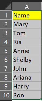
As you can see we have a column with 9 observations and we want each of these observations to repeat 8 times consecutively. So ‘Mary’ will repeat for 8 times and then ‘Tom’ will start and repeat for 8 times and so on. Now let’s see what we can do here.
- We can copy the column in a separate sheet and then insert another column ‘Sum’ to the left of our original column ‘Name’ as you can see in the diagram below.
- Add another column ‘Repeat Times’ to the right of the column ‘Name’ and specify the number of times you want to repeat the observations e.g. 8 times in this case.
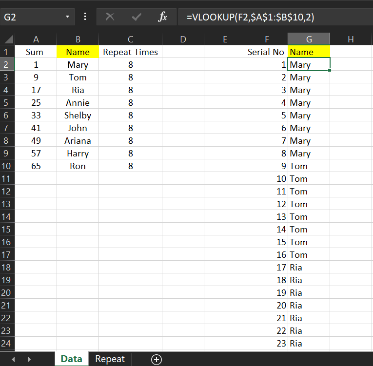
- Then come to column ‘Sum’ and put 1 in the first row A2.Then in the second row add A2 and C2 and drag down the formula. So basically in cell A3 it will be 1+8 =9; in A4 it will be 9+17 = 25 and so on.

Now finally we will do a simple VLOOKUP to get the desired output. See the diagram below.
- We create a column of serial numbers. Simply put 1 in the first row and in the second row add 1 with it. Drag it down and go till 65 because because 65 is final cumulative sum at the end cell (A10) of the column ‘Sum’. So we need to go till 65.
- In a column next to the serial no we will write a vlookup. The lookup value will be the serial number. The lookup array will be fixed. We will only select the range of the column sum and the column ‘Name. No need to include the column ‘repeat times’. Then we will put the column number of the column whose observations we want to repeat. In this case the column is ‘Name’ and hence, the number will be 2.That’s it. Simply drag it down till serial number 65 and you will get the desired result as shown below.
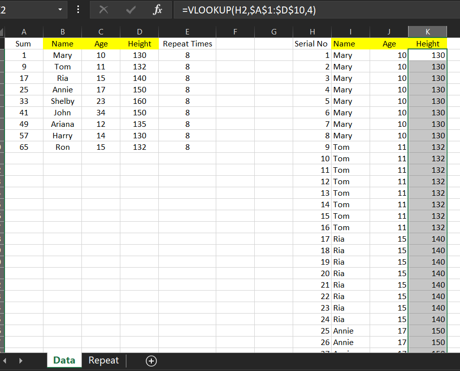
Please note that if we need to repeat this exercise for a number of columns i.e. suppose we have other columns ‘Age’ and ‘Height’ and so on. Simply add these columns next to column ‘Name’ and repeat the same Vlookup formula. Only the column number will be changed and the lookup array will include the new 2 columns . See the example below
For column ‘Age’ put the column number as 3 and for ‘height’ put the column number as 4.The lookup array is again fixed and include the range of values from A1:D10.
Hope you found this example helpful for your projects 🙂