What is normality?

Normality is a property of a random variable that follows normal probability distribution. A normal distribution has a zero mean with one standard deviation. In a graphical format, a ‘Normal’ distribution will appear as a bell curve, symmetric about the mean. In the Classical linear Regression model or in certain statistical tests, the assumption of normality refers to checking if our data roughly fits a bell curve shape in order to maintain consistency of the estimated coefficients.

Why do we care about normality?

First of all, let me start with why Normality is an important assumption. A primary reason for the normal distribution being important is that it is easy for Statisticians to work with. A lot of statistical tests assume normal distributions. However, these tests also work well if the underlying distribution is approximately normally distributed. Typically, in real life, we work with large samples (sample size > 30). For these cases, Central Limit Theorem kicks in which basically tells us the distribution of sample mean approximates a normal distribution as the sample size gets larger, regardless of the population’s distribution. Now let’s see how we can check for normality in a range of different samples.

6 ways to test for a normal distribution

Normality is not a required assumption for OLS estimation, however, non-normality may affect the results of hypothesis testing relying on normality assumptions. If this assumption is not satisfied, then we may see unreliable p values. In order to identify whether the error terms (residual) are normally distributed, multiple tests are performed, such as Anderson darling test, Kolmogorov Smirnov test, Shapiro Wilk test, and Jarque- Bera test, etc.

Passing criteria p>=0.05

Visual Methods:

1. Histogram

The first method that almost everyone knows is the histogram. The histogram is a data visualization that shows the distribution of a variable. It gives us the frequency of occurrence of each of the values in the dataset as per the user-defined bins or intervals. Histograms divide the data into bins of equal width. Each bin is plotted as a bar and the height of the bar depends on the frequency of the values in that bin. the diagram below shows an example of a histogram.

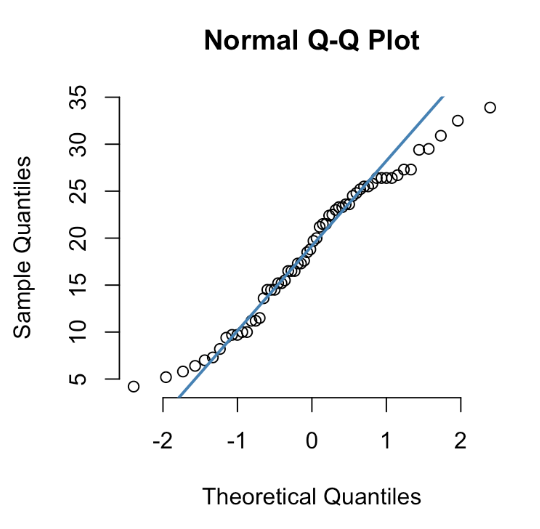
2. Q-Q plots

It plots two sets of quantiles against one another i.e., theoretical quantiles (of a normal distribution) against the actual quantiles of the variable. If our data comes from a normal distribution, we should see all the points sitting in a straight line. It is a non-parametric approach to compare two samples or to compare two theoretical distributions. QQ plots also help to identify outliers in the dataset. The below diagram shows an example of a QQ plot.

Statistical methods:

1. Shapiro Wilk Test

Usually, the Shapiro-Wilk test is appropriate for small sample sizes. It calculates a W statistic that tests whether a random sample comes from (specifically) a normal distribution. Small values of W indicate evidence of departure from normality. The values for the W statistic are obtained from Monte Carlo simulations.

Passing Criteria: The null hypothesis of this test is that the population is normally distributed. If the p-value is less than or equal to  0.05 (if alpha (chosen level of significance) = 5%) we can conclude that the data does not fit the normal distribution. If the p-value > 0.05, we can conclude that no significant departure from the normal distribution was observed. Obviously, the chosen level of significance varies based on the researcher.

2. Kolmogorv Smirnov Test

The difference between the cumulative proportions of the sample and the corresponding cumulative proportions from the normal distribution is computed and the absolute value of their maximum difference is reported. The Kolmogorov-Smirnov test computes the distances between the empirical distribution and the theoretical distribution and defines the test statistic as the maximum of those distances. The advantage of this is that the same approach can be used for comparing any distribution, not necessarily the normal distribution only. However, this test is less powerful than Shapiro Wilk test.

Passing Criteria: The null hypothesis is that both distributions are similar. So, if the p-value ≤ 0.05, then we reject the null hypothesis i.e. we assume the distribution does not follow a normal distribution. If the p-value > 0.05, then we fail to reject the null hypothesis.

3. Anderson Darling Test

The Anderson-Darling test is a modification of the Kolmogorov-Smirnov (K-S) test and gives more weight to the tails of the distribution than the K-S test hence, it is more powerful than KS test. This test is distribution-free in the sense that the critical values do not depend on the specific distribution being tested.

Passing Criteria: The null hypothesis is that both distributions are similar. So, if the p-value ≤ 0.05, then we reject the null hypothesis i.e. we assume the distribution does not follow a normal distribution. If the p-value > 0.05, then we fail to reject the null hypothesis.

Kolmogorov-Smirnov and Anderson-Darling tests are based on the assumption that Population mean and standard deviation are unknown and need to be estimated hence, they are known as EDF tests as they are based on the Empirical Distribution Function (EDF).

4. Jarque Bera Test

The Jarque-Bera test identifies normality based on the skewness and kurtosis of the time series. The Jarque-Bera Test is a type of Lagrange multiplier test. It tests whether a specific distribution matches the skewness and kurtosis of a normal distribution. It is usually used for large data sets because other normality tests are not reliable when number of observations is large (for example, Shapiro-Wilk isn’t reliable with n more than 2,000).

Passing Criteria: The null hypothesis is a joint hypothesis of both the skewness and the kurtosis being zero. Since the samples from a normal distribution have an expected skewness and an expected excess kurtosis of 0, if the p-value ≤ 0.05, then we reject the null hypothesis i.e. we assume the distribution of our variable is not normal. In simpler words, the null hypothesis for the test is that the data is normally distributed; the alternate hypothesis is that the data does not come from a normal distribution.

Conclusion: It is always recommended to add visual testing of normality along with a statistical test. Visual tests help us to identify outliers which can be a primary reason for non-normality. In real data, we are bound to come across non-normal distribution very often. However, it definitely should not be a matter of worry. We should try to investigate the underlying reason and it is always a good practice to use 2/3 tests simultaneously and see if it is passing any one of them.