WOE and IV: Key Techniques for Credit Scorecard Models

Weight of evidence (WOE) and Information Value (IV) are widely used techniques to screen variables in credit scorecard models. In this article, I will discuss the details of WOE and IV based on their purpose, use and method.

What is Weight of Evidence (WOE)?

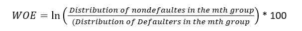
Since it evolved from credit scoring world, it is generally described as a measure of the separation of defaulters and non-defaulters. The formula of the weight of evidence (WOE) is as follows where distribution of non-defaulters is the % of Good customers or non-defaulters in ‘m’th group and distribution of defaulters is the % of Bad Customers in the same group.
Please note ‘ln’ is Natural Log in the formula below.

• Positive WOE means Distribution of Goods > Distribution of Bads
• Negative WOE means Distribution of Goods < Distribution of Bads
• Note: Log of a number > 1 means positive value. If less than 1, it means negative value.

Steps of Calculating WOE:

1. For a continuous variable, split data into 10 parts (or lesser depending on the distribution).
2. Calculate the number of events and non-events in each group (bin)
3. Calculate the % of events and % of non-events in each group.
4. Calculate WOE by taking natural log of division of % of non-events and % of events

Note : For a categorical variable, you do not need to split the data (Ignore Step 1 and follow the remaining steps)

The WOE values corresponding to the minimum default rate difference are used as WOE for the group containing missing values.

Fine Classing and Coarse Classing:

In the world of credit scoring, risk modeling, and feature engineering, each variable is investigated to determine the underlying defaulter/non-defaulter trends in the data. Once a trend is identified the fine classes are grouped together into coarser groups in order to smooth out fluctuations in continuous data and to achieve larger pools of similar risk. This process brings out the Information Values of the variables telling the ability of the variables to separate the defaulters and non-defaulters.

Information Value (IV):

WOE is often used alongside Information Value (IV), which measures the total predictive power of a variable:

• IV Interpretation:
  • < 0.02: Useless
  • 0.02–0.1: Weak predictor
  • 0.1–0.3: Medium predictor
  • > 0.3: Strong predictor

Applications:

1. Credit Risk Modeling
   • Banks use WOE to evaluate how categories like “Age Group” or “Income Level” predict loan defaults.
   • Example:
     • If “Age 30–40” has WOE = +0.5, this group is less likely to default.
     • If “Age < 25” has WOE = -0.8, this group is riskier.
2. Feature Engineering
   • Converts categorical variables into numerical WoE values for machine learning models (e.g., logistic regression).
3. Binning Continuous Variables
   • Groups continuous data (e.g., “Loan Amount”) into bins and calculates WoE for each bin.

Example Calculation:

Suppose we have a dataset of loan applicants:

Age Group	Non-Defaulters (Good)	Defaulters (Bad)	% Good	% Bad	WoE
<25	50	150	10%	30%	ln(10/30) = -1.10
25–40	300	200	60%	40%	ln(60/40) = +0.41
>40	150	150	30%	30%	ln(30/30) = 0

IV Calculation: IV=(0.1−0.3)×(−1.10)+(0.6−0.4)×0.41+(0.3−0.3)×0=0.302

Conclusion: “Age Group” is a strong predictor (IV > 0.3).

Advantages & Limitations

✅ Advantages:

• Handles non-linear relationships between categorical variables and target.
• Standardizes variables for better model interpretability.
• Robust to outliers (uses binning).

❌ Limitations:

• Requires careful binning (manual or optimal binning methods).
• Overfitting risk if bins are too granular.
• Only works for binary classification.

Key Takeaways

• WOE quantifies the relationship between a categorical variable and a binary outcome.
• IV evaluates the overall predictive power of a variable.
• Used in credit scoring, risk modeling, and feature engineering.
• Combines well with logistic regression and scorecard models.

Implementation in Python

import pandas as pd
import numpy as np

def calculate_woe_iv(df, feature, target, bins=10):
    # Bin the variable
    df['bin'] = pd.qcut(df[feature], bins, duplicates='drop')
    
    # Group by bin and calculate statistics
    grouped = df.groupby('bin')[target].agg(['count', 'sum'])
    grouped.columns = ['total', 'bads']
    grouped['goods'] = grouped['total'] - grouped['bads']
    
    # Total goods and bads
    total_goods = grouped['goods'].sum()
    total_bads = grouped['bads'].sum()
    
    # Calculate distribution and WOE
    grouped['dist_good'] = grouped['goods'] / total_goods
    grouped['dist_bad'] = grouped['bads'] / total_bads
    grouped['woe'] = np.log(grouped['dist_good'] / grouped['dist_bad']).replace([np.inf, -np.inf], 0)
    
    # IV
    grouped['iv'] = (grouped['dist_good'] - grouped['dist_bad']) * grouped['woe']
    
    # Final IV
    iv = grouped['iv'].sum()

    return grouped[['woe', 'iv']], iv


# Sample data
data = pd.DataFrame({
    'age': [25, 45, 35, 50, 23, 52, 40, 60, 48, 33],
    'default': [0, 1, 0, 0, 1, 0, 1, 0, 1, 0]
})

woe_iv_table, iv_value = calculate_woe_iv(data, 'age', 'default', bins=3)

print(woe_iv_table)
print("Information Value (IV):", iv_value)